1 Quantum free scalar field
This chapter is a quick review of the theory of the quantum free scalar field.
Notation for space-time points: \[ \begin{gather*} x = (x^0, \vec{x}) = (x^0, x^1, x^2, x^3) \ . \end{gather*} \] Minkowski metric: \[ \begin{gather*} g_{\mu\nu} = \text{diag}(1,-1,-1,-1) \ . \end{gather*} \]
1.1 Field and ladder operators
The quantum free (real) scalar field \(\phi(x)\) with mass \(m\) is an Hermitian operator satisfying the Klein-Gordon equation: \[ \begin{gather*} (\partial^2 + m^2) \phi(x) = 0 \ , \end{gather*} \tag{1.1}\] which is solved by going to momentum space: \[ \begin{gather*} \phi(x) = \int \frac{d^3p}{(2\pi)^3 2 E(\vec{p})} \left[ a(\vec{p}) e^{-i E(\vec{p}) x_0 + i \vec{p} \vec{x}} + a(\vec{p})^\dag e^{i E(\vec{p}) x_0 - i \vec{p} \vec{x}} \right] \ , \end{gather*} \tag{1.2}\] where \(E(\vec{p}) = \sqrt{m^2 + \vec{p}^2}\) is the energy of the free particle with momentum \(\vec{p}\). The canonical momentum is defined as: \[ \begin{gather*} \pi(x) = \partial_0 \phi(x) \ . \end{gather*} \tag{1.3}\]
Equal-time canonical commutation relations \[ \begin{align*} & [\phi(t,\vec{x}), \pi(t,\vec{y})] = i \delta^3(\vec{x} - \vec{y}) \ , \\ & [\phi(t,\vec{x}), \phi(t,\vec{y})] = [\pi(t,\vec{x}), \pi(t,\vec{y})] = 0 \ . \end{align*} \tag{1.4}\] are equivalent to the canonical commutation relations for the creation and annihilation operators: \[ \begin{align*} & [a(\vec{p}), a(\vec{q})^\dag] = 2 E(\vec{p}) (2\pi)^3 \delta^3(\vec{p} - \vec{q}) \ , \\ & [a(\vec{p}), a(\vec{q})] = [a(\vec{p})^\dag, a(\vec{q})^\dag] = 0 \ . \end{align*} \tag{1.5}\] Notice that we are using the so-called relativistic normalization for the creation and annihilation operators.
1.2 Multi-particle states
The vacuum state \(| \Omega \rangle\) is defined as the state annihilated by all the annihilation operators: \[ \begin{gather*} a(\vec{p}) | \Omega \rangle = 0 \ , \quad \text{for all } \vec{p} \ . \end{gather*} \tag{1.6}\] The vacuum state is interpreted as the state with no particles. Multi-particle states are constructed by acting with the creation operators on the vacuum state.
The state of a single particle with definite momentum \(\vec{p}\) (the wavefunction is a plane wave) is defined as: \[ \begin{gather*} | \vec{p} \rangle = a(\vec{p})^\dag | \Omega \rangle \ . \end{gather*} \tag{1.7}\] General \(n\)-particle states with definite momenta are defined as: \[ \begin{gather*} | \vec{p}_1, \vec{p}_2, \dots, \vec{p}_n \rangle = a(\vec{p}_1)^\dag a(\vec{p}_2)^\dag \cdots a(\vec{p}_n)^\dag | \Omega \rangle \ . \end{gather*} \tag{1.8}\] Notice that, thanks to the commutation relations, the order of the creation operators does not matter: by changing the order of the momenta we obtain the same state.
It is convenient to introduce the number-of-particles operator or, simply, the number operator: \[ \begin{gather*} N = \int \frac{d^3p}{(2\pi)^3 2 E(\vec{p})} \, a(\vec{p})^\dag a(\vec{p}) \ . \end{gather*} \tag{1.9}\] The vacuum and \(n\)-particle states introduced above are eigenstates of the number-of-particles operator: \[ \begin{align*} & N | \Omega \rangle = 0 \ , \\ & N | \vec{p}_1, \vec{p}_2, \dots, \vec{p}_n \rangle = n | \vec{p}_1, \vec{p}_2, \dots, \vec{p}_n \rangle \ . \end{align*} \tag{1.10}\]
Any possible state of the system can be written as a linear combination of the vacuum and multi-particle states, as in: \[ \begin{gather*} | \Psi \rangle = \Psi_0 \, | \Omega \rangle + \sum_{n=1}^\infty \frac{1}{n!} \int \left[ \prod_{k=1}^n \frac{d^3p_k}{(2\pi)^3 2 E(\vec{p}_k)} \right] \, \Psi_n(\vec{p}_1, \dots, \vec{p}_n) \, | \vec{p}_1, \dots, \vec{p}_n \rangle \ . \end{gather*} \tag{1.11}\] The set of normalizable states of this form constitute the Hilbert space \(\mathcal{H}\) of the free scalar field, which is also called the Fock space. The set of states with definite particle number equal to \(n\) (i.e. the set of eigenstates of \(N\) with eigenvalue \(n\)) is called the \(n\)-particle sector of the Fock space \(\mathcal{H}_n\). The \(0\)-particle sector is also called vacuum sector. One can define orthogonal projectors on the \(n\)-particle sectors: \[ \begin{align*} & \mathbb{P}_0 = | \Omega \rangle \langle \Omega | \ , \\ & \mathbb{P}_1 = \int \frac{d^3p}{(2\pi)^3 2 E(\vec{p})} \, | \vec{p} \rangle \langle \vec{p} | \ , \\ & \mathbb{P}_n = \frac{1}{n!} \int \left[ \prod_{k=1}^n \frac{d^3p_k}{(2\pi)^3 2 E(\vec{p}_k)} \right] \, | \vec{p}_1, \dots, \vec{p}_n \rangle \langle \vec{p}_1, \dots, \vec{p}_n | \ . \end{align*} \tag{1.12}\] The completeness relation on the Fock space reads: \[ \begin{gather*} \sum_{n=0}^\infty \mathbb{P}_n = 1 \ . \end{gather*} \tag{1.13}\]
1.3 Four-momentum and invariant-mass operators
The energy-momentum tensor can be obtained by means of Noether’s theorem from the invariance of the action under space-time translations and it reads: \[ \begin{gather*} T^{\mu\nu} = \partial^\mu \phi \partial^\nu \phi - g^{\mu\nu} \left( \frac{1}{2} \partial_\rho \phi \partial^\rho \phi - \frac{1}{2} m^2 \phi^2 \right) + \epsilon_0 g^{\mu\nu} \ , \end{gather*} \tag{1.14}\] where \(\epsilon_0\) is an arbitrary constant. A change of \(\epsilon_0\) corresponds to a change of the vacuum energy density. The Hamiltonian operator \(H=P^0\) and the momentum operator \(\vec{P}\) are obtained by integrating the energy-momentum tensor: \[ \begin{gather*} P^\mu = \int d^3x \, T^{0\mu}(x_0,\vec{x}) \ . \end{gather*} \tag{1.15}\] From the right-hand side it may seem that \(P^\mu\) depends on \(x_0\). However, by using the conservation of the energy-momentum tensor, i.e. \[ \begin{gather*} \partial_\mu T^{\mu\nu}(x) = 0 \ , \end{gather*} \tag{1.16}\] one can show that \(P^\mu\) does not depend on \(x_0\), i.e. it is conserved.
The four-momentum operator can be easily written in terms of the creation and annihilation operators: \[ \begin{align*} & H = \int \frac{d^3p}{(2\pi)^3 2 E(\vec{p})} \, E(\vec{p}) \, a(\vec{p})^\dag a(\vec{p}) \ , \\ & \vec{P} = \int \frac{d^3p}{(2\pi)^3 2 E(\vec{p})} \, \vec{p} \, a(\vec{p})^\dag a(\vec{p}) \ , \end{align*} \tag{1.17}\] with an appropriate choice of the constant \(\epsilon_0\). The four-momentum operator is the generator of translations, in particular \[ \begin{gather*} e^{-i a_\mu P^\mu} \, \phi(x) \, e^{i a_\mu P^\mu} = \phi(x - a) \ . \end{gather*} \tag{1.18}\] This equation can be also written in infinitesimal form: \[ \begin{gather*} i [ P^\mu, \phi(x) ] = \partial^\mu \phi(x) \ . \end{gather*} \tag{1.19}\]
Let us introduce an auxiliary real parameter \(s\) and consider the following expression: \[ \begin{gather*} \phi_s(x) = e^{-i s a_\mu P^\mu} \, \phi(x) \, e^{i s a_\mu P^\mu} \ . \end{gather*} \] The operator \(\phi_s(x)\) satisfies the following differential equation: \[ \begin{gather*} \frac{d}{ds} \phi_s(x) = -i a_\rho e^{-i s a_\mu P^\mu} \, [ P_\rho , \phi(x) ] \, e^{i s a_\mu P^\mu} \ , \end{gather*} \] with initial condition \(\phi_0(x) = \phi(x)\). Using the expression of the field in terms of the creation and annihilation operators and the commutation relations, one easily finds that: \[ \begin{gather*} [ P_\rho , \phi(x) ] = -i \partial_\rho \phi(x) \ , \end{gather*} \] therefore the differential equation can be written equivalently as: \[ \begin{gather*} \frac{d}{ds} \phi_s(x) = - a_\rho \partial_\rho \phi_s(x) \ . \end{gather*} \] The solution of this equation is: \[ \begin{gather*} \phi_s(x) = \phi(x - s a) \ , \end{gather*} \] where we have used the initial condition \(\phi_0(x) = \phi(x)\). By choosing \(s=1\) and using the definition of \(\phi_s(x)\) we obtain the desired result.
Using the commutation relations, one shows that the components of the four-momentum operator commute with each other. In particular this means that they can be simultaneously diagonalized. The vacuum and the multi-particle states are eigenstates of the four-momentum operator: \[ \begin{align*} & P^\mu | \Omega \rangle = 0 \ , \\ & H | \vec{p}_1, \vec{p}_2, \dots, \vec{p}_n \rangle = \left[ \sum_{k=1}^n E(\vec{p}_k) \right] \, | \vec{p}_1, \vec{p}_2, \dots, \vec{p}_n \rangle \ , \\ & \vec{P} | \vec{p}_1, \vec{p}_2, \dots, \vec{p}_n \rangle = \left[ \sum_{k=1}^n \vec{p}_k \right] \, | \vec{p}_1, \vec{p}_2, \dots, \vec{p}_n \rangle \ . \end{align*} \tag{1.20}\]
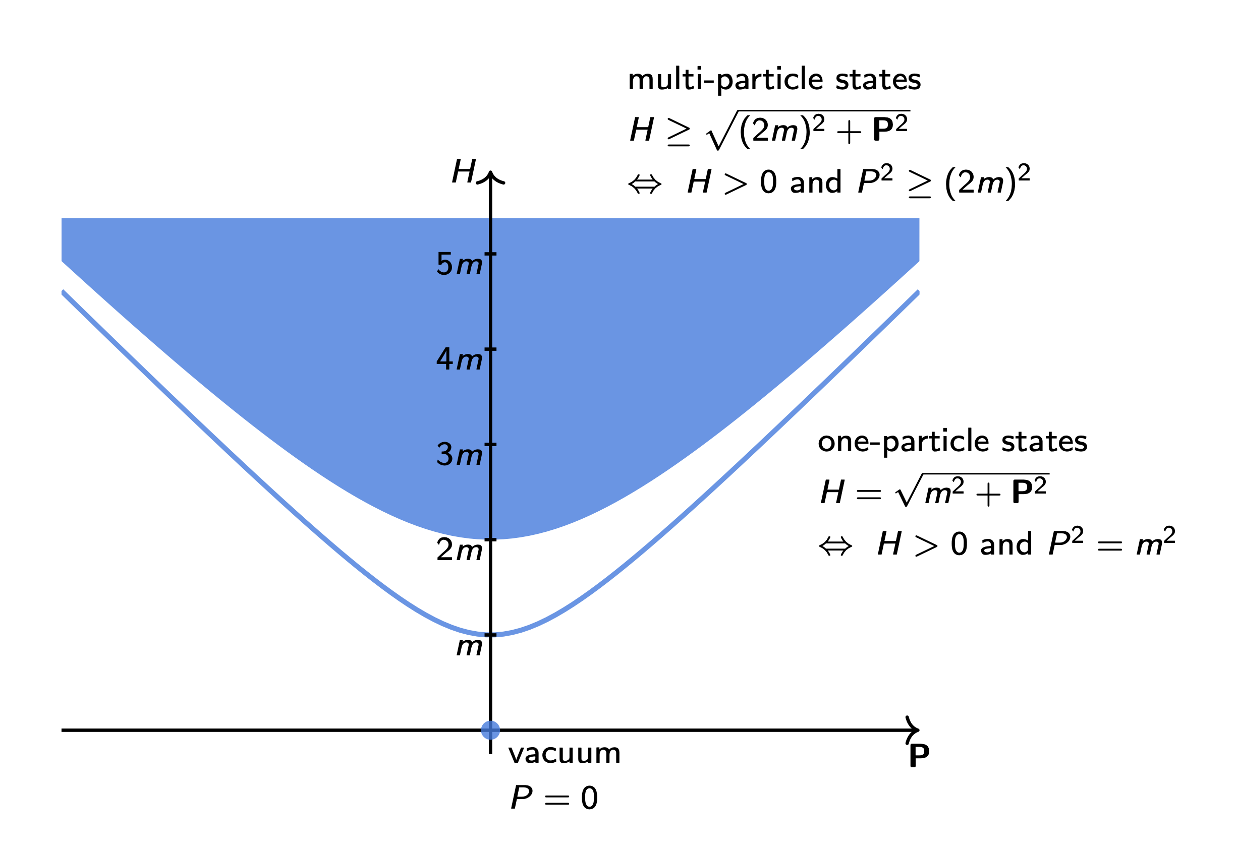
In the vacuum sector, the four-momentum operator has a single eigenvalue, which is zero. In the \(1\)-particle sector, the spectrum of the four-momentum operator is given by the set of all possible on-shell momenta of a free particle with mass \(m\). We will denote such set as: \[ \begin{gather*} \mathcal{M}_1 = \{ p \in \mathbb{R}^4 \text{ s.t. } p^2 = m^2 \text{ and } p_0 > 0 \} \ . \end{gather*} \tag{1.21}\] Notice that this set is a subset of the forward open light cone, i.e. the set of all time-like four-momenta with positive time component: \[ \begin{gather*} \mathcal{M}_1 \subset \Lambda^+ = \{ p \in \mathbb{R}^4 \text{ s.t. } p^2 > 0 \text{ and } p_0 > 0 \} \ . \end{gather*} \tag{1.22}\] In the \(n\)-particle sector for \(n \ge 2\), the spectrum of the four-momentum operator is given by the set of all possible sums of on-shell momenta of \(n\) free particles with mass \(m\): \[ \begin{gather*} \mathcal{M}_{n \ge 2} = \left\{ \sum_{k=1}^n p_k \text{ s.t. } p_{1,\dots,n} \in \mathcal{M}_1 \right\} = \left\{ p \in \mathbb{R}^4 \text{ s.t. } p^2 \ge (n \times m)^2 \text{ and } p_0 > 0 \right\} \ . \end{gather*} \tag{1.23}\] The proof of the last equality is left as an exercise for the reader. It follows that the set \(\mathcal{M}_2\) contains the set \(\mathcal{M}_n\) for all \(n \ge 2\). Therefore, the spectrum of the four-momentum operator for the free scalar field is given simply by \(\{0\} \cup \mathcal{M}_1 \cup \mathcal{M}_2\), which can be written as: \[ \begin{gather*} \sigma(P) = \{0\} \cup \left\{ p \in \Lambda^+ \text{ s.t. } p^2 = m^2 \right\} \cup \left\{ p \in \Lambda^+ \text{ s.t. } p^2 \ge (2m)^2 \right\} \ . \end{gather*} \tag{1.24}\] A visualization of the spectrum of the four-momentum operator is given in figure Figure 1.1.
The invariant-mass operator (or, simply, mass operator) is defined as: \[ \begin{gather*} M = \sqrt{P^2} = \sqrt{P_\mu P^\mu} = \sqrt{H^2 - \vec{P}^2} \ . \end{gather*} \tag{1.25}\] The square root is well defined because the eigenvalues of \(P\) are either zero or time-like, which meant that \(P^2\) is non-negative. The spectrum of the invariant-mass operator is easily calculated from the spectrum of the four-momentum operator: \[ \begin{gather*} \sigma(M) = \{0\} \cup \{ m \} \cup [2m, +\infty) \ . \end{gather*} \tag{1.26}\] Notice that it contains two discrete eigenvalues (corresponding to the vacuum and the \(1\)-particle states) and a continuous part (corresponding to the \(n\)-particle states with \(n \ge 2\)).
1.4 Problems
Download Matthew Black’s solutions.
Problem 1.1 Starting from the commutation relations for the ladder operators, show that \([ \phi(x) , \phi(y) ] = 0\) if \((x-y)\) is space-like. This is the so-called microcausality property of the free scalar field.
Problem 1.2 Prove that the components of the four-momentum operator commute with each other.
Problem 1.3 Prove that the operators \(\mathbb{P}_n\) are mutually orthogonal projectors on the \(n\)-particle sector of the Fock space.
Problem 1.4 Prove that the states \(| \vec{p}_1, \vec{p}_2, \dots, \vec{p}_n \rangle\) are eigenstates of the four-momentum and calculate their eigenvalues.
Problem 1.5 Prove that \[ \begin{gather*} \left\{ p_1 + p_2 \text{ s.t. } p_1, p_2 \in \mathcal{M}_1 \right\} = \left\{ p \in \mathbb{R}^4 \text{ s.t. } p^2 \ge (2 m)^2 \text{ and } p_0 > 0 \right\} \ . \end{gather*} \]
Problem 1.6 Prove that the following operator \[ \begin{gather*} L^{\mu\nu} = \int d^3x \, [ x^\nu T^{0\mu}(x) - x^\mu T^{0\nu}(x) ] \end{gather*} \] does not depend on \(x^0\) and that it generates Lorentz transformations on the field \(\phi(x)\). In particular, for any real matrix \(\omega_{\mu\nu}\) satisfying \(\omega_{\mu\nu} = - \omega_{\nu\mu}\), show that: \[ \begin{gather*} e^{-\frac{i}{2} \omega_{\mu\nu} L^{\mu\nu}} \, \phi(x) \, e^{\frac{i}{2} \omega_{\mu\nu} L^{\mu\nu}} = \phi(\Lambda^{-1} x) \end{gather*} \] where \(\Lambda = e^\omega\) is a Lorentz transformation.