3 One-particle states
When talking about scattering in particle physics one has in mind the following situation:
at a certain time in the far past (in the idealized case, at \(t = -\infty\)), two particles are prepared very far apart from each other and with velocities such that they move towards each other;
as the particles approach each other, they interact possibly in a very complicated way; a number of particles is produced (they may be different from the particles in the initial state);
the particles in the final state move away from each other and are detected at a certain time in the far future (in the idealized case, at \(t = +\infty\)).
The initial and final states (at \(t = \pm \infty\)) are called asymptotic states, whose construction is one of the main topics of this course. However, before getting there, we need to reflect on a seemingly trivial yet crucial point: the particles in the asymptotic states must be infinitely far apart from each other. This means that we are not allowed to consider the individual particles in states with a definite momentum, as these states are plane waves and therefore completely delocalized in space: two particles in a state with definite momentum are never apart from each other. Asymptotic states should be constructed in terms of one-particle (1P) states with wave functions which are localized in space, usually called wave packets. In this lecture we will discuss the construction of such 1P states in a generic interacting QFT and their properties.
3.1 Normalizable 1P states
We consider a QFT satisfying the properties described in chapter Chapter 2. For simplicity, we consider the case in which a single scalar particle exists with mass \(m\). In this case, Equation 2.17 specializes to \[ \begin{gather*} \langle \vec{p}' | \vec{p} \rangle = 2 E(\vec{p}) (2\pi)^3 \delta^3(\vec{p} - \vec{p}') \ . \end{gather*} \tag{3.1}\] The projector onto the one-particle subspace is defined as \[ \begin{gather*} \hat{P}_1 = \int \frac{d^3 p}{(2\pi)^3 2 E(\vec{p})} \, |\vec{p}\rangle \langle \vec{p}| \ . \end{gather*} \tag{3.2}\] The one-particle state with wavefunction \(\hat{f}(\vec{p})\) is defined as \[ \begin{gather*} | f \rangle = \int \frac{d^3 p}{(2\pi)^3 2 E(\vec{p})} \, \hat{f}(\vec{p}) \, |\vec{p}\rangle \ . \end{gather*} \tag{3.3}\] We will consider only smooth wavefunctions with compact support.1 In particular, we choose some some energy scale \(\lambda > 0\) and we consider only wavefunctions \(\hat{f}(\vec{p})\) which vanish for \(|\vec{p}| \ge \lambda\). This is not a fundamental restriction, since \(\lambda\) can be chosen arbitrarily large. The normalization condition for the state \(| f \rangle\) is \[ \begin{gather*} \langle f | f \rangle = \int \frac{d^3 p}{(2\pi)^3 2 E(\vec{p})} \, |\hat{f}(\vec{p})|^2 = 1 \ . \end{gather*} \tag{3.4}\] The time evolution of the state \(| f \rangle\) is given by \[ \begin{gather*} e^{-iHt} | f \rangle = \int \frac{d^3 p}{(2\pi)^3 2 E(\vec{p})} \, \hat{f}(\vec{p}) \, e^{-iE(\vec{p})t} |\vec{p}\rangle = | f_t \rangle \ , \end{gather*} \tag{3.5}\] with the definition \[ \begin{gather*} \hat{f}_t(\vec{p}) = e^{-iE(\vec{p})t} \hat{f}(\vec{p}) \ . \end{gather*} \tag{3.6}\]
3.1.1 Weak localization property at finite time
We want to argue heuristically that the state \(| f_t \rangle\) can be thought as essentially localized in space for every \(t\). To this end, we consider the inverse Fourier transform of the wavefunction \(\hat{f}_t(\vec{p}) / \sqrt{ 2 E(\vec{p}) }\) i.e. \[ \begin{gather*} f_t(\vec{x}) = \int \frac{d^3 p}{(2\pi)^3 \sqrt{ 2 E(\vec{p}) }} \, e^{i \vec{p} \vec{x}} \, \hat{f}_t(\vec{p}) = \int \frac{d^3 p}{(2\pi)^3 \sqrt{ 2 E(\vec{p}) }} \, e^{-iE(\vec{p})t + i \vec{p} \vec{x}} \, \hat{f}(\vec{p}) \ . \end{gather*} \tag{3.7}\] The reason for the unusual factor \(1 / \sqrt{ 2 E(\vec{p}) }\) lies in the fact that the states \(|\vec{p}\rangle\) are defined with relativistic normalization. A way to check that the above definition makes sense is to check that the \(L^2\) norm of the function \(f_t(\vec{x})\) coincides with norm of the state \(| f \rangle\). In fact, using standard properties of the Fourier transform, we find \[ \begin{gather*} \int d^3 x \, | f_t(\vec{x}) |^2 = \int \frac{d^3 p}{(2\pi)^3} \left| \frac{\hat{f}_t(\vec{p})}{\sqrt{ 2 E(\vec{p}) }} \right|^2 = \int \frac{d^3 p}{(2\pi)^3 2 E(\vec{p})} \, |\hat{f}(\vec{p})|^2 = \langle f | f \rangle \end{gather*} \tag{3.8}\] Since the wavefunction \(\hat{f}_t(\vec{p})\) is smooth with compact support, so is the function \(\hat{f}_t(\vec{p}) / \sqrt{ 2 E(\vec{p}) }\). In particular, \(\hat{f}_t(\vec{p}) / \sqrt{ 2 E(\vec{p}) }\) is Schwartz and, therefore, its inverse Fourier transform \(f_t(\vec{x})\) is also Schwartz (see for instance the Wikipedia article on Schwartz functions and references therein). One can prove that, if \(\hat{f}(\vec{p})\) is not identically zero, then the function \(f_t(\vec{x})\) does not have a compact support for any \(t\).2 Therefore \(f_t(\vec{x})\) is not localized in a strict sense, but simply in the sense that it decays fast for large values of \(\vec{x}\). We will say that \(f_t(\vec{x})\) is localized in a weak sense.
In order to build some intuition about the time-evolution of the wavefunction \(f_t(\vec{x})\), is it interesting to analyze how the average position and the width of the wave function (or position indetermination) evolve in time. Interpreting the function \(f_t(\vec{x})\) as a wavefunction in position space, and taking inspiration from the textbook Quantum Mechanical point particle, we can define the average position \(\bar{\vec{x}}(t)\) and position indetermination \(\Delta x(t)\) by means of the following equations: \[ \begin{align*} & \bar{\vec{x}}(t) = \int d^3 x \, \vec{x} \, | f_t(\vec{x}) |^2 \ , \\ & \Delta x^2(t) = \int d^3 x \, [ \vec{x} - \bar{\vec{x}}(t) ]^2 \, | f_t(\vec{x}) |^2 \ , \end{align*} \tag{3.9}\] where we have assumed, with no loss of generality, that the state \(| f \rangle\) is normalized, i.e. \(\langle f | f \rangle = 1\). Recall that the velocity \(\vec{v}\) of a relativistic particle in uniform motion is related to the momentum \(\vec{p}\) by the relation \(\vec{v} = \vec{p} / E(\vec{p})\). Therefore, it makes sense to define the average velocity \(\bar{\vec{v}}(t)\) and the velocity indetermination \(\Delta v(t)\) as: \[ \begin{align*} & \bar{\vec{v}}(t) = \int \frac{d^3 p}{(2\pi)^3} \, \frac{\vec{p}}{E(\vec{p})} \, \left| \frac{\hat{f}_t(\vec{p})}{\sqrt{ 2 E(\vec{p}) }} \right|^2 = \bar{\vec{v}}(0) \equiv \bar{\vec{v}} \ , \\ & \Delta v^2(t) = \int \frac{d^3 p}{(2\pi)^3} \, \left[ \frac{\vec{p}}{E(\vec{p})} - \bar{\vec{v}}(t) \right]^2 \, \left| \frac{\hat{f}_t(\vec{p})}{\sqrt{ 2 E(\vec{p}) }} \right|^2 = \Delta v^2(0) \equiv \Delta v^2 \ , \end{align*} \tag{3.10}\] where we have used the fact that \(| \hat{f}_t(\vec{p}) |\) does not depend on \(t\). By expressing \(f_t(\vec{x})\) in terms of the momentum-space wavefunction \(\hat{f}(\vec{p})\) in Equation 3.9 and using standard properties of the Fourier transform, one can make the time dependence of the average position and the position indetermination explicit: \[ \begin{align*} & \bar{\vec{x}}(t) = \bar{\vec{x}}(0) + \bar{\vec{v}} \, t \ , \\ & \Delta x^2(t) = \Delta x^2(0) + D \, t + \Delta v^2 \, t^2 \ , \end{align*} \tag{3.11}\] where \(D\) is a sort of diffusion coefficient. Notice that the average position moves like the position of a classical particle in uniform motion with constant velocity \(\bar{\vec{v}}\). At large time, the position indetermination \(\Delta x(t)\) grows like \(t\), which is a typical feature of a quantum particle in uniform motion.
3.2 Creation operators for 1P states
We want to show that the state \(| f \rangle\) can be obtained from the vacuum state \(| \Omega \rangle\) by acting with a suitably-defined creation operator \(\hat{a}(f)^\dag\), which is a linear functional of the wavefunction \(\hat{f}(\vec{p})\) and the field operators. The construction of such a creation operator in an interacting QFT is a non-trivial task and requires a number of steps.
3.2.1 Interpolating field and normalization factor
Let \(\phi(x)^\dag\) be an interpolating field for the particle with mass \(m\), as discussed in Section 2.2. Since we are considering a scalar particle, \(\phi(x)\) must be a scalar field operator. We observe that matrix element \(\langle \vec{p} | \phi(x)^\dag | \Omega \rangle\) is generally a tempered distribution in \(x\) and \(\vec{p}\). However, the \(x\) dependence is fixed by the observation that \[ \begin{gather*} \langle \vec{p} | \phi(x)^\dag | \Omega \rangle = \langle \vec{p} | e^{iPx} \phi(0)^\dag e^{-iPx} | \Omega \rangle = e^{i E(\vec{p}) x_0 - i \vec{p} \vec{x}} \langle \vec{p} | \phi(0)^\dag | \Omega \rangle \ . \end{gather*} \tag{3.12}\] A boost \(\Lambda_{\vec{p}}\) exists from the rest frame of the particle to a frame in which the particle has momentum \(\vec{p}\), i.e. \(U(\Lambda_{\vec{p}}) | \vec{0} \rangle = | \vec{p} \rangle\). Using the invariance of the vacuum under Lorentz transformations and the fact that the field \(\phi(x)^\dag\) is a scalar, we obtain \[ \begin{gather*} \langle \vec{p} | \phi(0)^\dag U(\Lambda_{\vec{p}}) | \Omega \rangle = \langle \vec{0} | U(\Lambda_{\vec{p}})^\dag \phi(0)^\dag U(\Lambda_{\vec{p}}) | \Omega \rangle = \langle \vec{0} | \phi(0)^\dag | \Omega \rangle \ , \end{gather*} \tag{3.13}\] i.e. the matrix element \(\langle \vec{p} | \phi(0)^\dag | \Omega \rangle\) is independent of \(\vec{p}\) and it is a constant, which is commonly denoted by \(Z^{1/2}\). Therefore, we can write \[ \begin{gather*} \langle \vec{p} | \phi(x)^\dag | \Omega \rangle = Z^{1/2} e^{i E(\vec{p}) x_0 - i \vec{p} \vec{x}} \ . \end{gather*} \tag{3.14}\]
3.2.2 The auxiliary function \(\tilde{\zeta}(\omega)\)
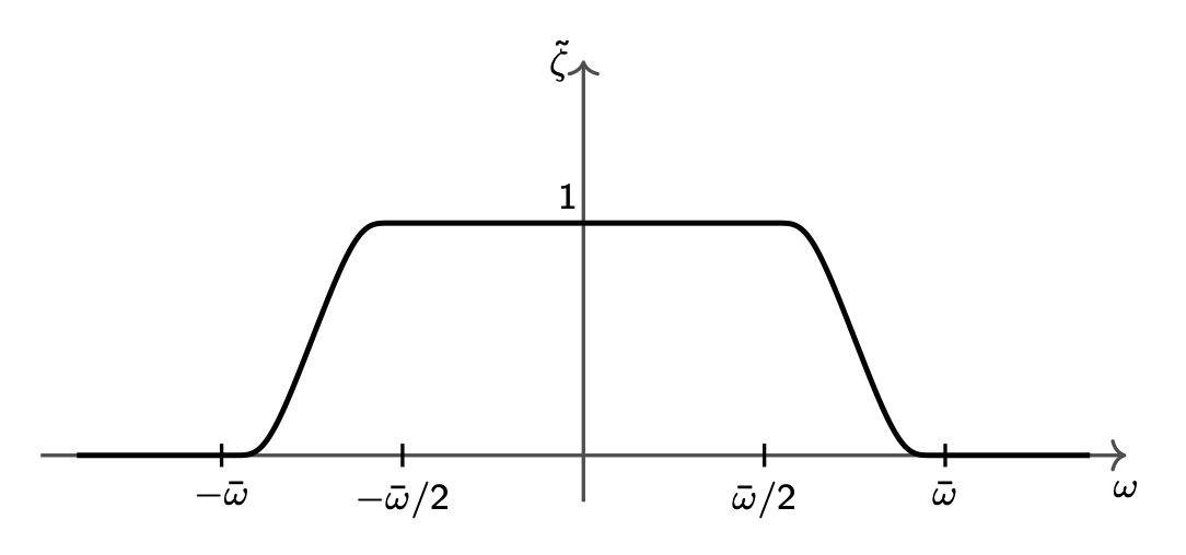
As discussed in Section 2.2, we assume that the spectrum of the invariant mass operator satisfies: \[ \begin{gather*} \sigma(M) \subseteq \{ 0 \} \cup \{ m \} \cup [ m + \Delta, +\infty ) \ , \end{gather*} \tag{3.15}\] where \(\Delta > 0\). With no loss of generality, we can assume that \(\Delta \le m\). Define \[ \begin{gather*} \bar{\omega} = \frac{ \sqrt{(m+\Delta)^2 + \lambda^2} - \sqrt{m^2 + \lambda^2} }{2} = \frac{ \Delta \left( m + \Delta/2 \right) }{ \sqrt{(m+\Delta)^2 + \lambda^2} + \sqrt{m^2 + \lambda^2} } \ . \end{gather*} \tag{3.16}\] Recall that we consider only wavefunctions \(\hat{f}(\vec{p})\) which vanish for \(|\vec{p}| \ge \lambda\). From the above expression, it is easy to prove that \(0 < \bar{\omega} < \frac{\Delta}{2} < \frac{m}{2}\). Let us consider a smooth function \(\tilde{\zeta}(\omega)\) with the following properties:
\(\tilde{\zeta}(\omega)\) vanishes for \(|\omega| \ge \bar{\omega}\);
\(\tilde{\zeta}(\omega) = 1\) for \(|\omega| \le \bar{\omega}/2\).
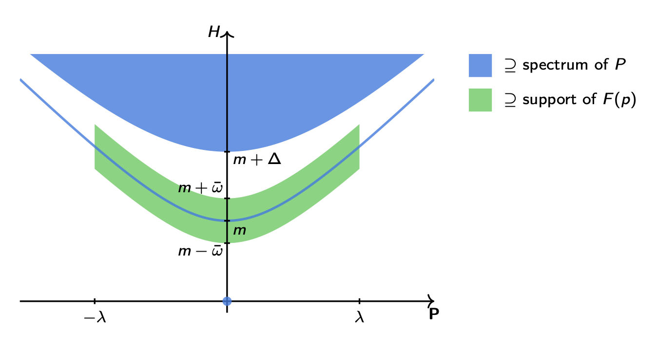
An explicit expression for \(\tilde{\zeta}(\omega)\) can be easily written in terms of the so-called smooth transition functions, described for instance in the Wikipedia article on bump functions. However such an explicit expression is not needed in the following. A pictorial representation of the function \(\tilde{\zeta}(\omega)\) is shown in Figure 3.1. We consider the following function: \[ \begin{gather*} F(p) = \hat{f}(\vec{p}) \, \tilde{\zeta}(p_0 - E(\vec{p}) ) \ , \end{gather*} \tag{3.17}\] which satisfies the following properties:
\(F(p)\) is smooth and has compact support;
the support of \(F(p)\), represented by the green shaded area in Figure 3.2, intersects the spectrum of the invariant mass operator \(\sigma(M)\) only on the one-particle mass-shell hyperboloid;
the restriction of \(F(p)\) to the mass-shell hyperboloid is equal to \(\hat{f}(\vec{p})\).
Notice that the role of the function \(\tilde{\zeta}(p_0 - E(\vec{p}) )\) is to cut off contributions of states that do not correspond to the one-particle states from the function \(F(p)\).
3.2.3 Creation operator and fundamental property
The creation operator \(\hat{a}(f)^\dag\) is defined as \[ \begin{gather*} a(f)^\dag = \frac{1}{Z^{1/2}} \int \frac{d^4 p}{(2\pi)^4} \, F(p) \, \tilde{\phi}(p)^\dag = \frac{1}{Z^{1/2}} \int \frac{d^4 p}{(2\pi)^4} \, \hat{f}(\vec{p}) \, \tilde{\zeta}(p_0 - E(\vec{p}) ) \, \tilde{\phi}(p)^\dag \ , \end{gather*} \tag{3.18}\] where \(\tilde{\phi}(p)\) is the Fourier transform of the field \(\phi(x)\), i.e. \[ \begin{gather*} \tilde{\phi}(p) = \int d^4 x \, e^{i p x} \, \phi(x) \ . \end{gather*} \tag{3.19}\] In order to being able to interpret the operator \(\hat{a}(f)^\dag\) as a creation operator, we need to check that it satisfies the following minimal property: \[ \begin{gather*} \hat{a}(f)^\dag | \Omega \rangle = | f \rangle \ . \end{gather*} \tag{3.20}\]
Let us see how this works. We start from the observation that \(\tilde{\phi}(p)^\dag | \Omega \rangle\) is an eigenstate of the energy-momentum operator \(P\) with eigenvalue \(p\). This is a consequence of Problem 2.2 and we are going to check it here in full detail. First we notice that \[ \begin{align*} e^{i P a} \tilde{\phi}(p)^\dag e^{-i P a} =& \int d^4 x \, e^{-i p x} \, e^{i P a} \phi(x)^\dag e^{-i P a} \\ = & \int d^4 x \, e^{-i p x} \, \phi(x+a)^\dag \\ = & \int d^4 x \, e^{-i p (x-a)} \, \phi(x)^\dag = e^{i p a} \tilde{\phi}(p)^\dag \ . \end{align*} \tag{3.21}\] By differentiating with respect to \(a^\mu\) and setting \(a = 0\), we find the commutation relation \[ \begin{align*} [ P_\mu , \tilde{\phi}(p)^\dag ] = & -i \left. \frac{\partial}{\partial a^\mu} \right|_{a=0} e^{i P a} \tilde{\phi}(p)^\dag e^{-i P a} \\ = & -i \left. \frac{\partial}{\partial a^\mu} \right|_{a=0} e^{i p a} \tilde{\phi}(p)^\dag = p_\mu \tilde{\phi}(p)^\dag \ . \end{align*} \tag{3.22}\] Finally, by acting on the vacuum, we get the eigenvalue equation for \(\tilde{\phi}(p)^\dag | \Omega \rangle\), i.e. \[ \begin{align*} P_\mu \tilde{\phi}(p)^\dag | \Omega \rangle = p_\mu \tilde{\phi}(p)^\dag | \Omega \rangle \ . \end{align*} \tag{3.23}\] Obviously, also \(F(p) \tilde{\phi}(p) | \Omega \rangle\) is an eigenstate of the energy-momentum operator \(P\) with eigenvalue \(p\). However, \(F(p)\) vanishes for values of \(p\) which correspond to eigenstates of \(P\) that are not one-particle states. Therefore, \(F(p) \tilde{\phi}(p) | \Omega \rangle\) is a linear combination of one-particle states, which implies: \[ \begin{align*} F(p) \tilde{\phi}(p)^\dag | \Omega \rangle = & \mathbb{P}_1 F(p) \tilde{\phi}(p)^\dag | \Omega \rangle \\ = & F(p) \int \frac{d^3 q}{(2\pi)^3 2 E(\vec{q})} \, | \vec{q} \rangle \langle \vec{q} | \tilde{\phi}(p)^\dag | \Omega \rangle \\ = & F(p) \int \frac{d^3 q}{(2\pi)^3 2 E(\vec{q})} \int d^4 x \, e^{-i p x} \, | \vec{q} \rangle \langle \vec{q} | \phi(x)^\dag | \Omega \rangle \\ = & Z^{1/2} F(p) \int \frac{d^3 q}{(2\pi)^3 2 E(\vec{q})} \, | \vec{q} \rangle \int d^4 x \, e^{-i [p_0 - E(\vec{q})] x_0 + i (\vec{p} - \vec{q} ) \vec{x}} \\ = & Z^{1/2} F(p) \int \frac{d^3 q}{(2\pi)^3 2 E(\vec{q})} \, | \vec{q} \rangle (2\pi)^4 \delta(p_0 - E(\vec{q})) \delta^3(\vec{p} - \vec{q}) \\ = & \frac{Z^{1/2} F(E(\vec{p}),\vec{p})}{2 E(\vec{q})} \, | \vec{p} \rangle \, 2\pi \delta(p_0 - E(\vec{p})) \ . \\ = & \frac{Z^{1/2} \hat{f}(\vec{p})}{2 E(\vec{q})} \, | \vec{p} \rangle \, 2\pi \delta(p_0 - E(\vec{p})) \ . \end{align*} \tag{3.24}\] In the above calculation we have used the properties for \(F(p)\) and Equation 3.14. Finally, by combining this result with the definition of the creation operator \(\hat{a}(f)^\dag\) in Equation 3.18, we find \[ \begin{align*} a(f)^\dag | \Omega \rangle = & \frac{1}{Z^{1/2}} \int d^4 p \, F(p) \, \phi(p)^\dag | \Omega \rangle \\ = & \frac{1}{Z^{1/2}} \int \frac{d^4 p}{(2\pi)^4} \, \frac{Z^{1/2} \hat{f}(\vec{p})}{2 E(\vec{q})} \, | \vec{p} \rangle \, 2\pi \delta(p_0 - E(\vec{p})) \\ = & \int \frac{d^3 p}{(2\pi)^3 2 E(\vec{p})} \, \hat{f}(\vec{p}) \, |\vec{p}\rangle = | f \rangle \ , \end{align*} \tag{3.25}\] which is the desired result in Equation 3.20.
3.2.4 Position space representation
It is interesting to notice that the creation operator can be expressed in terms of the field in position space. Expressions in position space will allow us to study the localization properties of states obtained by acting with products of creation operators on the vacuum. The most straightforward way to obtain such an expression is to express \(\tilde{\phi}(p)\) in Equation 3.18 in terms of the field \(\phi(x)\) in position space. However, we will follow a slightly more involved route, which will allow us to express the creation operator in terms of a smeared field. This is useful because smeared fields are smooth as a function of the coordinates and, therefore, easier to control mathematically.
We need to introduce a second auxiliary function \(\tilde{\eta}(\vec{p})\) with the following properties:
\(\tilde{\eta}(\vec{p})\) is a smooth function with compact support;
\(\tilde{\eta}(\vec{p}) = 1\) for \(|\vec{p}| \le \lambda\);
\(\tilde{\eta}(\vec{p}) = 0\) for \(|\vec{p}| \ge 2\lambda\).
\(\tilde{\eta}(\vec{p})\) plays the role of a cut-off function in the spatial momentum. In particular, one obtains the trivial identity \[ \begin{gather*} \hat{f}(\vec{p}) \tilde{\eta}(\vec{p}) = \hat{f}(\vec{p}) \ . \end{gather*} \tag{3.26}\] In fact, if \(|\vec{p}| \le \lambda\), the above equation holds because \(\tilde{\eta}(\vec{p}) = 1\) and, if \(|\vec{p}| > \lambda\), the above equation holds because \(\hat{f}(\vec{p}) = 0\) by assumption.
It is convenient to define the following combination of the two cut-off function \[ \begin{gather*} \tilde{\chi}(p)^* = \sqrt{2 E(\vec{p})} \, \tilde{\zeta}(p_0 - E(\vec{p}) ) \, \tilde{\eta}(\vec{p}) \ . \end{gather*} \tag{3.27}\] Using the properties of the two cut-off functions, we can easily check that \(\tilde{\chi}(p)\) is a smooth function with compact support which is identically equal to \(\sqrt{2 E(\vec{p})}\) in the green shaded area in Figure 3.2. The introduction of the factor \(\sqrt{2 E(\vec{p})}\) does not have a special meaning and it is simply a matter of convenience, as we will see below.
Introducing the above cut-off functions, the creation operator can be rewritten as \[ \begin{align*} a(f)^\dag = & \frac{1}{Z^{1/2}} \int \frac{d^4 p}{(2\pi)^4} \, \hat{f}(\vec{p}) \, \tilde{\eta}(\vec{p}) \, \tilde{\zeta}(p_0 - E(\vec{p}) ) \, \tilde{\phi}(p)^\dag \\ = & \frac{1}{Z^{1/2}} \int \frac{d^4 p}{(2\pi)^4} \, \frac{ \hat{f}(\vec{p}) }{ \sqrt{2 E(\vec{p})} } \, \tilde{\chi}(p)^* \, \tilde{\phi}(p)^\dag \ . \end{align*} \tag{3.28}\] Recalling that the Fourier transform maps the convolution in the porduct, we notice that \[ \begin{gather*} \tilde{\phi}^\chi(p) = \tilde{\chi}(p) \phi(p) \end{gather*} \tag{3.29}\] is nothing but the Fourier transform of the field smeared with the function \(\chi(x)\), which is defined as the inverse Fourier transform of \(\tilde{\chi}(p)\), i.e. \[ \begin{gather*} \phi^\chi(x) = \int d^4y \, \tilde{\chi}(x-y) \, \phi(y) \ . \end{gather*} \tag{3.30}\] Using this fact in Equation 3.28, we can rewrite the creation operator as \[ \begin{align*} a(f)^\dag = & \frac{1}{Z^{1/2}} \int \frac{d^4 p}{(2\pi)^4} \, \frac{ \hat{f}(\vec{p}) }{ \sqrt{2 E(\vec{p})} } \, \tilde{\phi}^\chi(p)^\dag \\ = & \frac{1}{Z^{1/2}} \int \frac{d^4 p}{(2\pi)^4} \, \frac{ \hat{f}(\vec{p}) }{ \sqrt{2 E(\vec{p})} } \, \int d^4 x \, e^{-i p x} \, \phi^\chi(x)^\dag \ . \end{align*} \tag{3.31}\] Notice that \(p_0\) appears only in the exponential, therefore the integral over \(p_0\) can be performed analytically and yields \(2\pi \delta(x_0)\). Integrating over \(x_0\), we find \[ \begin{gather*} a(f)^\dag = \frac{1}{Z^{1/2}} \int d^3x \int \frac{d^3 p}{(2\pi)^3 \sqrt{2 E(\vec{p})}} \, \hat{f}(\vec{p}) \, e^{i \vec{p} \vec{x}} \, \phi^\chi(0,\vec{x})^\dag \ . \end{gather*} \tag{3.32}\] Finally, thanks to the introduction of the factor \(\sqrt{2 E(\vec{p})}\), we can recognize that the integral over \(\vec{p}\) yields the function \(f_t(\vec{x})\) for \(t=0\). The function \(f_t(\vec{x})\) was introduced in Equation 3.7 and analyzed in Section 3.1.1. Our final expression for the creation operator in terms of the smeared field in position space is \[ \begin{gather*} a(f)^\dag = \frac{1}{Z^{1/2}} \int d^3x \, f_0(\vec{x}) \, \phi^\chi(0,\vec{x})^\dag \ . \end{gather*} \tag{3.33}\]
3.3 Problems
Download Matthew Black’s solutions.
Problem 3.1 Prove Equation 3.11 by using the definition of \(f_t(\vec{x})\) in Equation 3.7 and the properties of the Fourier transform and calculate the coefficient \(D\) in terms of the wavefunction \(\hat{f}(\vec{p})\).
Problem 3.2 Calculate the action of the Poincaré group on \(\tilde{\phi}(p)\), starting from Equation 2.11.
Problem 3.3 Prove that \[ \begin{gather*} e^{-iHt} a(f)^\dag | \Omega \rangle = a(f_t)^\dag | \Omega \rangle \ . \end{gather*} \]
Problem 3.4 Using arguments similar to those in Section 3.2.3, show that the operator \(a(f)\) annihilates the vacuum, i.e. \[ \begin{gather*} a(f) | \Omega \rangle = 0 \ . \end{gather*} \]
Problem 3.5 Calculate the matrix element \(\langle \vec{p} | \phi^\chi(x)^\dag | \Omega \rangle\) for the smeared field \(\phi^\chi(x)\), where \(\chi(x)\) is defined in Section 3.2.4.
Problem 3.6 Check that, in the case of the free theory, the creation operator \(a(f)^\dag\) defined in Equation 3.18 coincides with the creation operator defined in the free theory integrated against the wavefunction \(\hat{f}(\vec{p})\).
Problem 3.7 Consider the operator \[ \begin{gather*} A_t(f) = \frac{1}{Z^{1/2}} \int d^3x \, f_t(\vec{x}) \, \phi^\chi(t,\vec{x})^\dag \ . \end{gather*} \] Check that, in the case of the free theory, \(A_t(f)\) does not depend on \(t\).
Many results presented in these lecture can be generalized to Schwartz wavefunctions. In fact, many textbooks consider directly the Schwartz case. However, the assumption of compact support simplifies the presentation in a few points.↩︎
This follows from the fact that the integral in Equation 3.7 is holomorphic for every complex value of \(\vec{x}\). Therefore, for every \(\vec{x}_0\), the Taylor series of \(f_t(\vec{x})\) around \(\vec{x}_0\) converges everywhere in the complex plane and it is equal to \(f_t(\vec{x})\). If \(f_t(\vec{x})\) has a compact support, then we can choose \(\vec{x}_0\) away from the support of \(f_t(\vec{x})\) and the Taylor series around \(\vec{x}_0\) would be identically zero, which implies that \(f_t(\vec{x})\) is identically zero. This, in turn, implies that \(\hat{f}(\vec{p})\) is identically zero.↩︎